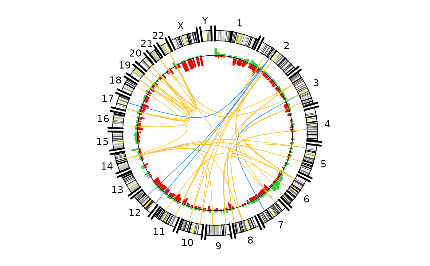
Plot a circular genome with aberration frequencies and connections between genomic loci added.

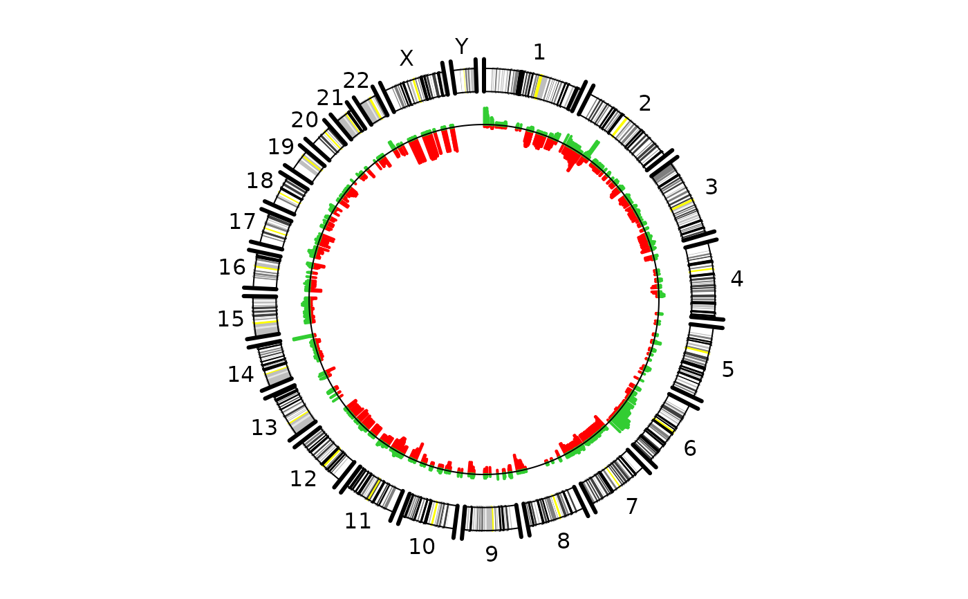
A circular genome is plotted and the percentage of samples that have a gain or a loss at a genomic position is added in the middle of the circle. Gains/losses correspond to copy number values that are above/below a pre-defined threshold. In addition arcs representing some connection between genomic loci may be added.

Usage

plotCircle(
  segments,
  thres.gain,
  thres.loss = -thres.gain,
  pos.unit = "bp",
  freq.colors = c("red", "limegreen"),
  alpha = 1/7,
  arcs = NULL,
  arc.colors = c("goldenrod1", "dodgerblue"),
  d = 0.3,
  assembly = "hg19"
)

Arguments

segments: a data frame containing the segmentation results found by either pcf() or multipcf().
thres.gain: a scalar giving the threshold value to be applied for calling gains.
thres.loss: a scalar giving the threshold value to be applied for calling losses. Default is to use the negative value of thres.gain.
pos.unit: the unit used to represent the probe positions. Allowed options are "mbp" (mega base pairs), "kbp" (kilo base pairs) or "bp" (base pairs). By default assumed to be "bp".
freq.colors: a vector giving the colors to be used for the amplification and deletion frequencies, respectively. Default is c("red","limegreen").
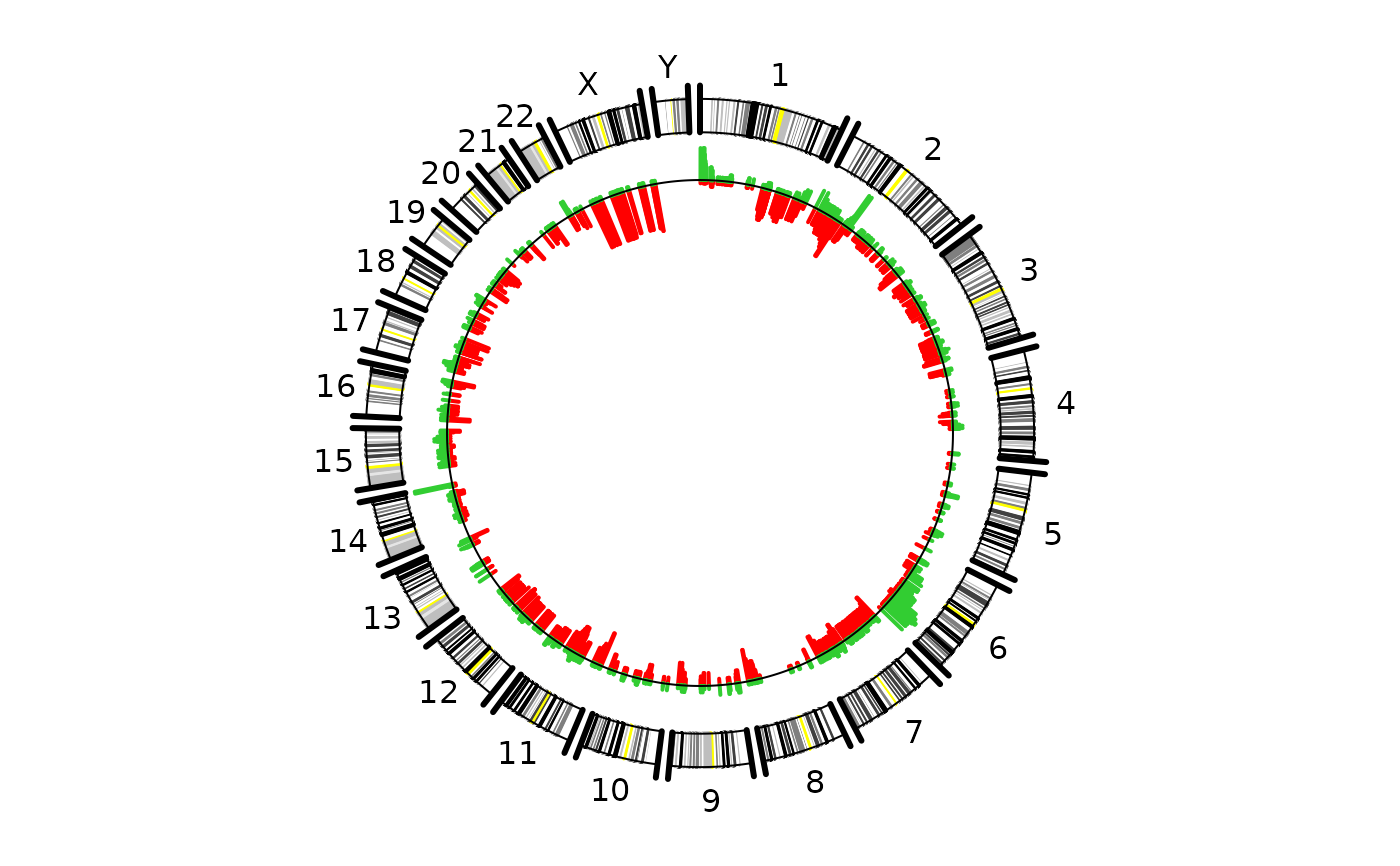
alpha: a scalar in the range 0 to 1 determining the amount of scaling of the aberration frequencies. For the default value of 1/7 the distance between the genome circle and the zero-line of the frequency-circle corresponds to an aberration percentage of 100 %. See details.
arcs: an optional matrix or data frame with 5 columns specifying connections between genomic loci. The first two columns must give the chromosome numbers and local positions for the start points of the arcs, while the two next columns give the chromosome numbers and local positions for the end point of arcs. The last column should contain a vector of numbers 1,2,... indicating that the arcs belong to different classes. Each class of arcs will then be plotted in a different color.
arc.colors: a vector giving the colors to be used for plotting the different classes of arcs. Cannot be shorter than the number of unique classes in arcs. The first color will represent the first class in arcs, the second color the second class and so on.
d: a scalar > 0 representing the distance from the genome circle to the starting points of the arcs. Set d=0 to make arcs start at the genome circle.
assembly: a string specifying which genome assembly version should be applied to determine chromosome ideograms. Allowed options are "hg19", "hg18", "hg17" and "hg16" (corresponding to the four latest human genome annotations in the UCSC genome browser).

Details

To zoom in on the observed aberration frequencies one may increase alpha. However, the user should be aware that this implies that the distance between the genome circle and the frequency zero-line does not reflect an aberration frequency of 100 %. Since the distance between the two circles is always 1/7, the maximum plotted percentage will be 100/(alpha*7) and any percentages that are higher than this will be truncated to this value.

Author

Gro Nilsen

Examples


#load lymphoma data
data(lymphoma)
#Run pcf
pcf.res <- pcf(data=lymphoma,gamma=12)
#> pcf finished for chromosome arm 1p 
#> pcf finished for chromosome arm 1q 
#> pcf finished for chromosome arm 2p 
#> pcf finished for chromosome arm 2q 
#> pcf finished for chromosome arm 3p 
#> pcf finished for chromosome arm 3q 
#> pcf finished for chromosome arm 4p 
#> pcf finished for chromosome arm 4q 
#> pcf finished for chromosome arm 5p 
#> pcf finished for chromosome arm 5q 
#> pcf finished for chromosome arm 6p 
#> pcf finished for chromosome arm 6q 
#> pcf finished for chromosome arm 7p 
#> pcf finished for chromosome arm 7q 
#> pcf finished for chromosome arm 8p 
#> pcf finished for chromosome arm 8q 
#> pcf finished for chromosome arm 9p 
#> pcf finished for chromosome arm 9q 
#> pcf finished for chromosome arm 10p 
#> pcf finished for chromosome arm 10q 
#> pcf finished for chromosome arm 11p 
#> pcf finished for chromosome arm 11q 
#> pcf finished for chromosome arm 12p 
#> pcf finished for chromosome arm 12q 
#> pcf finished for chromosome arm 13q 
#> pcf finished for chromosome arm 14q 
#> pcf finished for chromosome arm 15q 
#> pcf finished for chromosome arm 16p 
#> pcf finished for chromosome arm 16q 
#> pcf finished for chromosome arm 17p 
#> pcf finished for chromosome arm 17q 
#> pcf finished for chromosome arm 18p 
#> pcf finished for chromosome arm 18q 
#> pcf finished for chromosome arm 19p 
#> pcf finished for chromosome arm 19q 
#> pcf finished for chromosome arm 20p 
#> pcf finished for chromosome arm 20q 
#> pcf finished for chromosome arm 21q 
#> pcf finished for chromosome arm 22q 
#> pcf finished for chromosome arm 23p 
#> pcf finished for chromosome arm 23q 

plotCircle(segments=pcf.res,thres.gain=0.1)


#Use alpha to view the frequencies in more detail:
plotCircle(segments=pcf.res,thres.gain=0.1,alpha=1/5)


#An example of how to specify arcs
#Using multipcf, we compute the correlation between all segments and then
#retrieve those that have absolute inter-chromosomal correlation > 0.7
multiseg <- multipcf(lymphoma)
#> multipcf finished for chromosome arm 1p 
#> multipcf finished for chromosome arm 1q 
#> multipcf finished for chromosome arm 2p 
#> multipcf finished for chromosome arm 2q 
#> multipcf finished for chromosome arm 3p 
#> multipcf finished for chromosome arm 3q 
#> multipcf finished for chromosome arm 4p 
#> multipcf finished for chromosome arm 4q 
#> multipcf finished for chromosome arm 5p 
#> multipcf finished for chromosome arm 5q 
#> multipcf finished for chromosome arm 6p 
#> multipcf finished for chromosome arm 6q 
#> multipcf finished for chromosome arm 7p 
#> multipcf finished for chromosome arm 7q 
#> multipcf finished for chromosome arm 8p 
#> multipcf finished for chromosome arm 8q 
#> multipcf finished for chromosome arm 9p 
#> multipcf finished for chromosome arm 9q 
#> multipcf finished for chromosome arm 10p 
#> multipcf finished for chromosome arm 10q 
#> multipcf finished for chromosome arm 11p 
#> multipcf finished for chromosome arm 11q 
#> multipcf finished for chromosome arm 12p 
#> multipcf finished for chromosome arm 12q 
#> multipcf finished for chromosome arm 13q 
#> multipcf finished for chromosome arm 14q 
#> multipcf finished for chromosome arm 15q 
#> multipcf finished for chromosome arm 16p 
#> multipcf finished for chromosome arm 16q 
#> multipcf finished for chromosome arm 17p 
#> multipcf finished for chromosome arm 17q 
#> multipcf finished for chromosome arm 18p 
#> multipcf finished for chromosome arm 18q 
#> multipcf finished for chromosome arm 19p 
#> multipcf finished for chromosome arm 19q 
#> multipcf finished for chromosome arm 20p 
#> multipcf finished for chromosome arm 20q 
#> multipcf finished for chromosome arm 21q 
#> multipcf finished for chromosome arm 22q 
#> multipcf finished for chromosome arm 23p 
#> multipcf finished for chromosome arm 23q 
nseg = nrow(multiseg)
cormat = cor(t(multiseg[,-c(1:5)]))
chr.from <- c()
pos.from <- c()
chr.to <- c()
pos.to <- c()
cl <- c()

thresh = 0.7
for (i in 1:(nseg-1)) {
  for (j in (i+1):nseg) {
    #Check if segment-correlation is larger than threshold and that the two
    #segments are located on different chromosomes
    if (abs(cormat[i,j]) > thresh && multiseg$chrom[i] != multiseg$chrom[j]) {
      chr.from = c(chr.from,multiseg$chrom[i])
      chr.to = c(chr.to,multiseg$chrom[j])
      pos.from = c(pos.from,(multiseg$start.pos[i] + multiseg$end.pos[i])/2)
      pos.to = c(pos.to,(multiseg$start.pos[j] + multiseg$end.pos[j])/2)
      if(cormat[i,j] > thresh){
        cl <- c(cl,1)           #class 1 for those with positive correlation
      }else{
        cl <- c(cl,2)           #class 2 for those with negative correlation
      }
    }
  }
}

arcs <- cbind(chr.from,pos.from,chr.to,pos.to,cl)

#Plot arcs between segment with high correlations; positive correlation in
#orange, negative correlation in blue:
plotCircle(segments=pcf.res,thres.gain=0.15,arcs=arcs,d=0)