An overview of the copynumber package • copynumber

Introduction

This document gives an overview and demonstration of the copynumber package, which provides tools for the segmentation and visualization of copy number data. In the analysis of such data a goal is to detect and locate areas of the genome with copy number abberations. This may help identify genes that are critical to the development and progression of cancer. To locate areas or segments of equal copy numbers, our methods make Piecewise Constant Fits to the data through penalized least squares minimization (Nilsen et al., 2012). That is, piecewise constant curves are fitted to the data by minimizing the distance between the curve and the observed data, while imposing a penalty for each discontinuity in the curve. Segmentation may be done on a single sample, simultaneously on several samples or simultaneously on different data tracks.

This is a fork of the archived Bioconductor package, adding support for more recent genome builds. See the GitHub repository for source and issues.

Overview

The diagram below gives an overview of the copynumber package and illustrates the natural workflow. Each part of this workflow is described below.

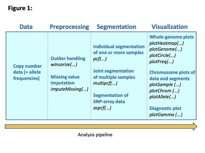
An overview of the copynumber package.

Data input

The data input in the copynumber package is normalized and log-transformed copy number measurements, for one or several samples. Allele-frequencies may also be specified for the segmentation of SNP-array data.

The data should be organized as a data matrix where each row represents a probe, and the first two columns give the chromosomes and genomic positions (locally in the chromosome) corresponding to each probe. Subsequent columns should hold the copy number measurements for each sample, and the header of these sample columns should be a sample identifier. For SNP-array data two such data matrices are required; one holding the LogR copy numbers and the other holding the B-allele frequencies (BAF).

Preprocessing

Outlier handling

Outliers are common in copy number data, and may have a substantial negative effect on the segmentation results. It is therefore strongly recommended to detect and modify extreme observations prior to segmentation. In the package we do this by Winsorization, and the method winsorize is available for this purpose.

Imputation of missing data

The method imputeMissing may be used for the imputation of missing copy number measurements. The user may decide on imputation by a constant or by an estimate based on the pcf-value (see below) of the nearest non-missing probes.

Segmentation

Segmentation tools

The copynumber package provides three segmentation tools. The method pcf handles the single-sample case, where segmentation is done independently for each sample in the data set, and the break points thus differ from sample to sample. The method multipcf runs on multiple samples simultaneously, and fits segmentation curves with common break points for all samples. The segment values will for each sample be equal to its average measurement on the segment. The third method, aspcf, is intended for SNP array data and performs allele-specific segmentation. This results in segmentation curves where break points are common for LogR and BAF data in the individual samples.

Choose model parameters

The most important parameter to set in the segmentation routines is gamma, which determines the penalty to be applied for each discontinuity or break point in the segmentation curve. Note that the default value will not be appropriate for all data sets; it may depend on the purpose of the study and artifacts may arise from the experimental procedure. Hence it is typically necessary to test a number of gamma values to find the optimal one. A valuable tool in this context is the diagnostic tool plotGamma, where segmentation is run for 10 different values of gamma and results are then displayed in a multigrid plot. This allows the user to explore the appropriateness of each segmentation result. Another parameter that influences the segmentation result is kmin, which imposes a minimum length (number of probes) for each segment.

Visualization

Several tools are available in the package for the plotting of data and segmentation results. These include plotGenome, plotSample, and plotChrom where data and/or segments are plotted over the entire genome, for a given sample across different chromosomes and for a given chromosome across different samples, respectively. Other graphical tools include plotHeatmap, which plots copy numbers heatmaps, and plotFreq, which plots the frequency of samples with an aberration at a genomic position. In addition, plotCircle enables the plotting of the genome as a circle with aberration frequencies and connections between genomic loci added to the middle of the circle.

Data sets

The package includes three data sets that are used in the examples below:

lymphoma: 3K aCGH data for a subset of 21 samples (Eide et al., 2010).
micma: A subset of a 244K aCGH data set. Contains data on chromosome 17 for 6 samples (Mathiesen et al., 2011).
logR and BAF: Artificial 10K SNP array data for 2 samples.

Examples

The following examples illustrate some applications of the copynumber package. First, load the package in R:

library(copynumber)

Single-sample segmentation

In this example we will use the lymphoma data:

data(lymphoma)

The data set has chromosomes and probe positions in the two first columns, and the copy number measurements for 21 samples in the subsequent columns. In this example we will only use a subset containing the first 3 samples, which corresponds to three biopsies from one patient taken at different time points. We can use the function subsetData to retrieve the desired data subset:

sub.lymphoma <- subsetData(data = lymphoma, sample = 1:3)
sub.lymphoma[1:10, ]

##    Chrom Median.bp  X01.B1  X01.B2  X01.B3
## 1      1   1082138  0.0906 -0.0144  0.0255
## 2      1   3318085 -0.0992 -0.1693 -0.0908
## 3      1   4552927 -0.0884 -0.0807  0.0401
## 4      1   5966170 -0.0503 -0.0231 -0.1081
## 5      1   7134999 -0.0970 -0.0145 -0.1877
## 6      1   7754220 -0.0671 -0.0291 -0.0506
## 7      1   9211391 -0.0386 -0.1290 -0.0058
## 8      1  10134471 -0.0281 -0.0507 -0.6507
## 9      1  11054335 -0.0231 -0.0520 -0.5539
## 10     1  11562778 -0.0780 -0.0742 -0.0531

Next we identify and modify outliers by the function winsorize:

lymph.wins <- winsorize(data = sub.lymphoma, verbose = FALSE)

The parameter verbose = FALSE just keeps the function from printing a progress message each time the analysis is finished for a new chromosome arm. The primary output from winsorize is then a new data frame (lymph.wins) on the same format as the input data where the sample columns now contain the Winsorized data values:

lymph.wins[1:10, ]

##    chrom      pos  X01.B1  X01.B2  X01.B3
## 1      1  1082138  0.0284 -0.0144  0.0255
## 2      1  3318085 -0.0992 -0.1693 -0.0908
## 3      1  4552927 -0.0884 -0.0807  0.0401
## 4      1  5966170 -0.0503 -0.0231 -0.1081
## 5      1  7134999 -0.0970 -0.0145 -0.1877
## 6      1  7754220 -0.0671 -0.0291 -0.0506
## 7      1  9211391 -0.0386 -0.1290 -0.0058
## 8      1 10134471 -0.0281 -0.0507 -0.2938
## 9      1 11054335 -0.0231 -0.0520 -0.3034
## 10     1 11562778 -0.0780 -0.0742 -0.0531

In addition, if the parameter return.outliers is set to TRUE, the method also returns a data frame which shows which observations have been classified as outliers:

wins.res <- winsorize(data = sub.lymphoma, return.outliers = TRUE, verbose = FALSE)
wins.res$wins.outliers[1:10, ]

##    chrom      pos X01.B1 X01.B2 X01.B3
## 1      1  1082138      1      0      0
## 2      1  3318085      0      0      0
## 3      1  4552927      0      0      0
## 4      1  5966170      0      0      0
## 5      1  7134999      0      0      0
## 6      1  7754220      0      0      0
## 7      1  9211391      0      0      0
## 8      1 10134471      0      0     -1
## 9      1 11054335      0      0     -1
## 10     1 11562778      0      0      0

The values 1 and -1 indicate outliers, reflecting that the original observation has been truncated to a smaller and higher value, respectively. The value 0 indicates that the observation is not an outlier and that the Winsorized value is identical to the original value. Note that one may obtain the winsorized data values in this setting by wins.res$wins.data.

Next we want to fit segmentation curves to each of the samples in our data using the function pcf. When Winsorization has been done, the Winsorized data should be the input (if one wants the segment values to equal the means of the observed data instead of the Winsorized data, one may in addition give the original data as input via the parameter Y = sub.lymphoma). The penalty parameter gamma is in this case set to 12 to achieve high sensitivity on these low-resolution data.

single.seg <- pcf(data = lymph.wins, gamma = 12, verbose = FALSE)

The default output of pcf is a data frame with 7 columns giving information about each segment found in the data. SampleIDs are given in the first column. Below we see the first six segments found in the subset of lymphoma samples:

head(single.seg)

##   sampleID chrom arm start.pos   end.pos n.probes    mean
## 1   X01.B1     1   p   1082138  64194749       70 -0.0455
## 2   X01.B1     1   p  65355304 119515493       58  0.0450
## 3   X01.B2     1   p   1082138  50340843       56 -0.0442
## 4   X01.B2     1   p  50638118 119515493       72  0.0219
## 5   X01.B3     1   p   1082138 119515493      128 -0.0329
## 6   X01.B1     1   q 142174575 146617392        8  0.0120

After the segmentation one may plot the data along with the segmentation results to see how well the segmentation fits the data. To plot the copy number data and the segmentation results over the entire genome we apply the function plotGenome, as illustrated below for one of the samples.

plotGenome(data = sub.lymphoma, segments = single.seg, sample = 1, cex = 3)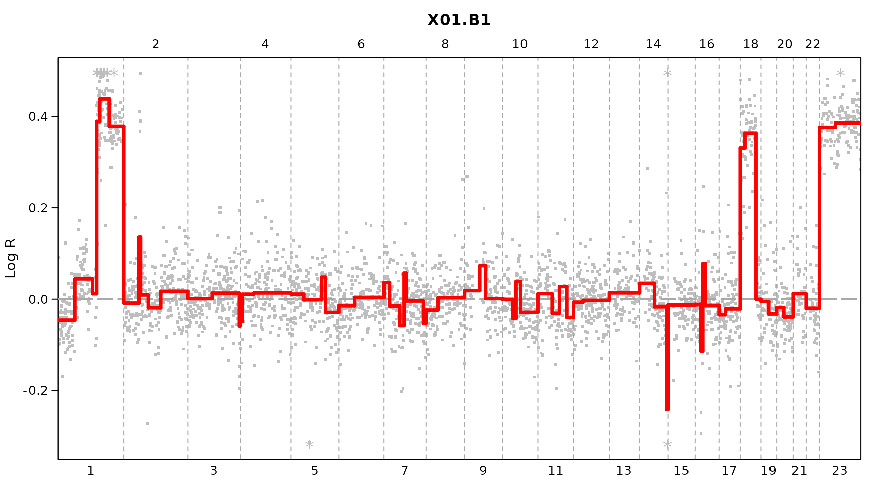

Genome plot for the sample X01.B1. Segmentation done by pcf.

Another plotting option is plotSample, where the data and segmentation results are shown for one sample with chromosomes in different panels. This is shown for the first sample below. Chromosome ideograms are by default added to the bottom of the plots.

plotSample(data = sub.lymphoma, segments = single.seg, layout = c(5, 5), sample = 1, cex = 3)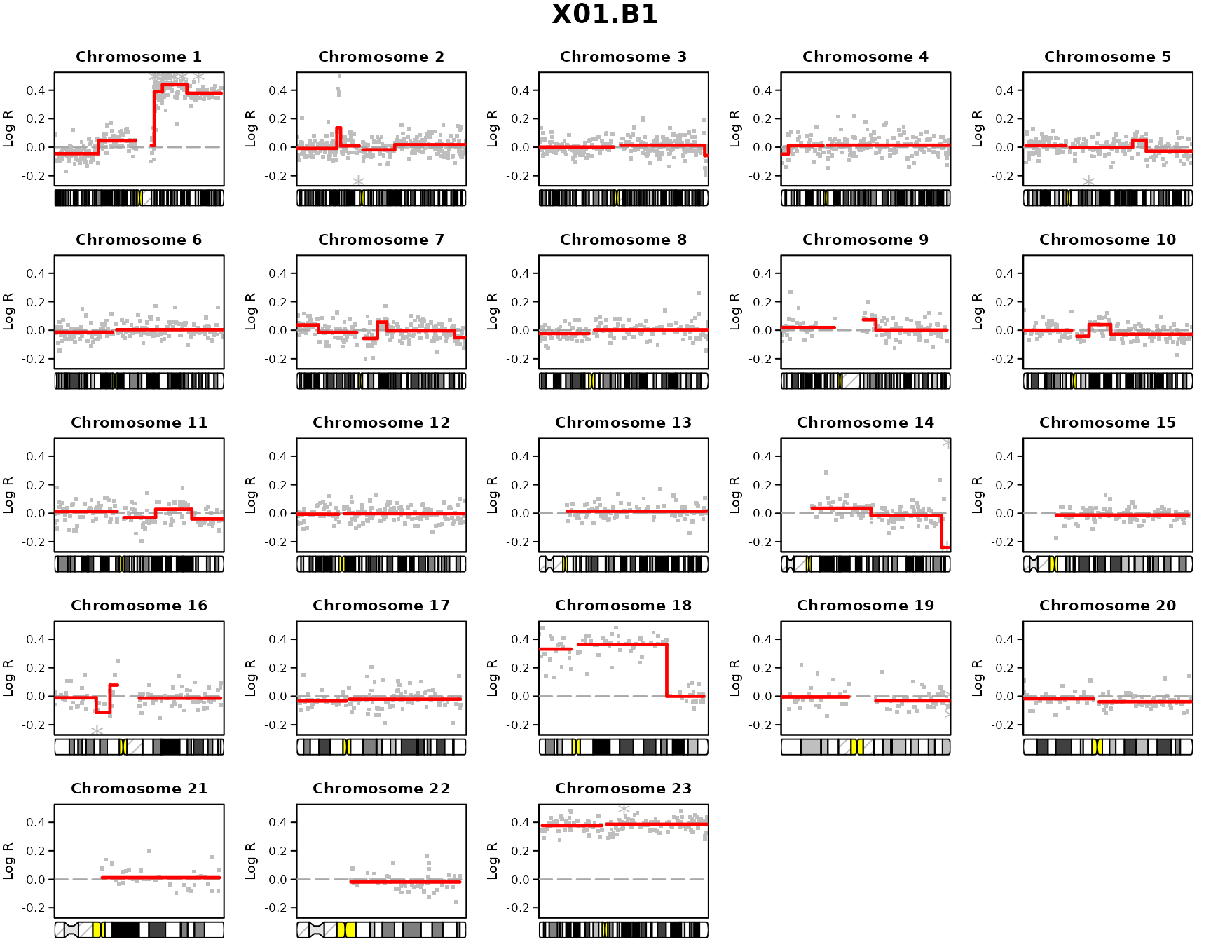

Sample X01.B1 plotted across the 23 chromosomes. Segmentation done by pcf.

Multi-sample segmentation

In the second example we illustrate multi-sample segmentation using the function multipcf on the three successive biopsies for sample X01. Input parameters and the output is similar to that of pcf, but the data frame holding the segmentation results now have common rows for all samples since they all have common segment boundaries:

multi.seg <- multipcf(data = lymph.wins, verbose = FALSE)
head(multi.seg)

##   chrom arm start.pos   end.pos n.probes  X01.B1  X01.B2  X01.B3
## 1     1   p   1082138  64194749       70 -0.0455 -0.0336 -0.0376
## 2     1   p  65355304 119515493       58  0.0450  0.0251 -0.0272
## 3     1   q 142174575 146617392        8  0.0120  0.0495 -0.0317
## 4     1   q 146756663 245340016      129  0.4038  0.0263 -0.0091
## 5     2   p    314759  89830600      107  0.0026  0.0004  0.0175
## 6     2   q  94941109 242568229      159  0.0063  0.0111  0.0061

To compare the segmentation results between samples we may use the function plotChrom. Here data and segments are plotted for one chromosome with samples in different panels, as illustrated below.

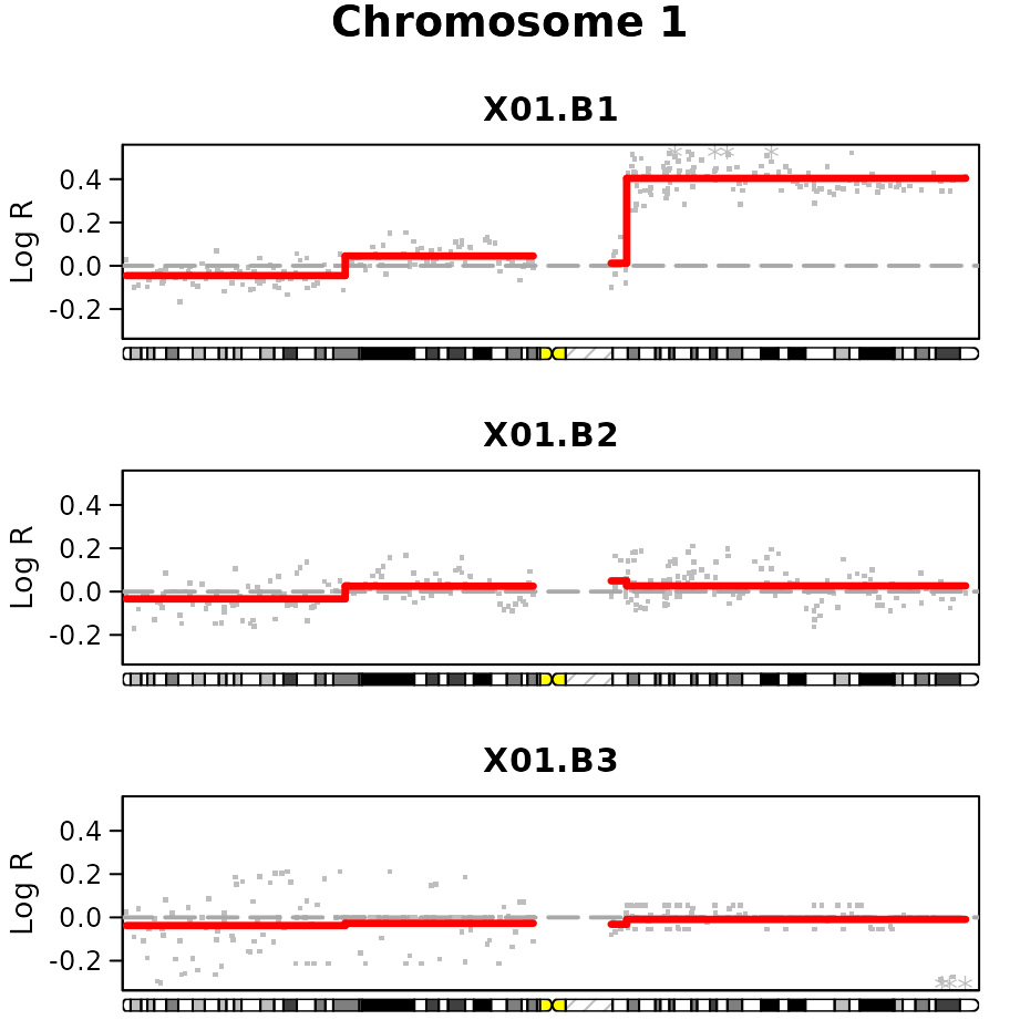
plotChrom(data = lymph.wins, segments = multi.seg, layout = c(3, 1), chrom = 1)

Chromosome 1 plotted for the 3 biopsies taken at different time points for sample X01. Segmentation done by multipcf.

Allele-specific segmentation

To illustrate allele-specific segmentation, we apply the artificial SNP-array data set containing both LogR data and BAF data:

data(logR)
data(BAF)

We start by Winsorizing the LogR data:

logR.wins <- winsorize(logR, verbose = FALSE)

The function aspcf will perform the allele-specific segmentation, taking both (Winsorized) LogR data and BAF data as input:

allele.seg <- aspcf(logR.wins, BAF, verbose = FALSE)
head(allele.seg)

##   sampleID chrom arm start.pos   end.pos n.probes logR.mean BAF.mean
## 1       S1     1   p   1695590  31067347      139   -0.2323   0.6916
## 2       S1     1   p  31101268  39640990       37    0.4000   0.7182
## 3       S1     1   p  39831894  46296225       34    0.1785   0.6207
## 4       S1     1   p  46437972  57577691       46    0.0289   0.5000
## 5       S1     1   p  57905199  60306875        9   -0.1552   0.6856
## 6       S1     1   p  60607571 100552011      128    0.0797   0.5000

Note that the output is similar to that of pcf, except for an extra 8’th column giving the segment BAF-values.

The function plotAllele may be used to plot the data and the segmentation results. For a given sample the results are shown for both the LogR- and BAF-track with chromosomes in different panels, as illustrated below for the first sample on chromosomes 1-4.

plotAllele(logR, BAF, allele.seg, sample = 1, chrom = c(1:4), layout = c(2, 2))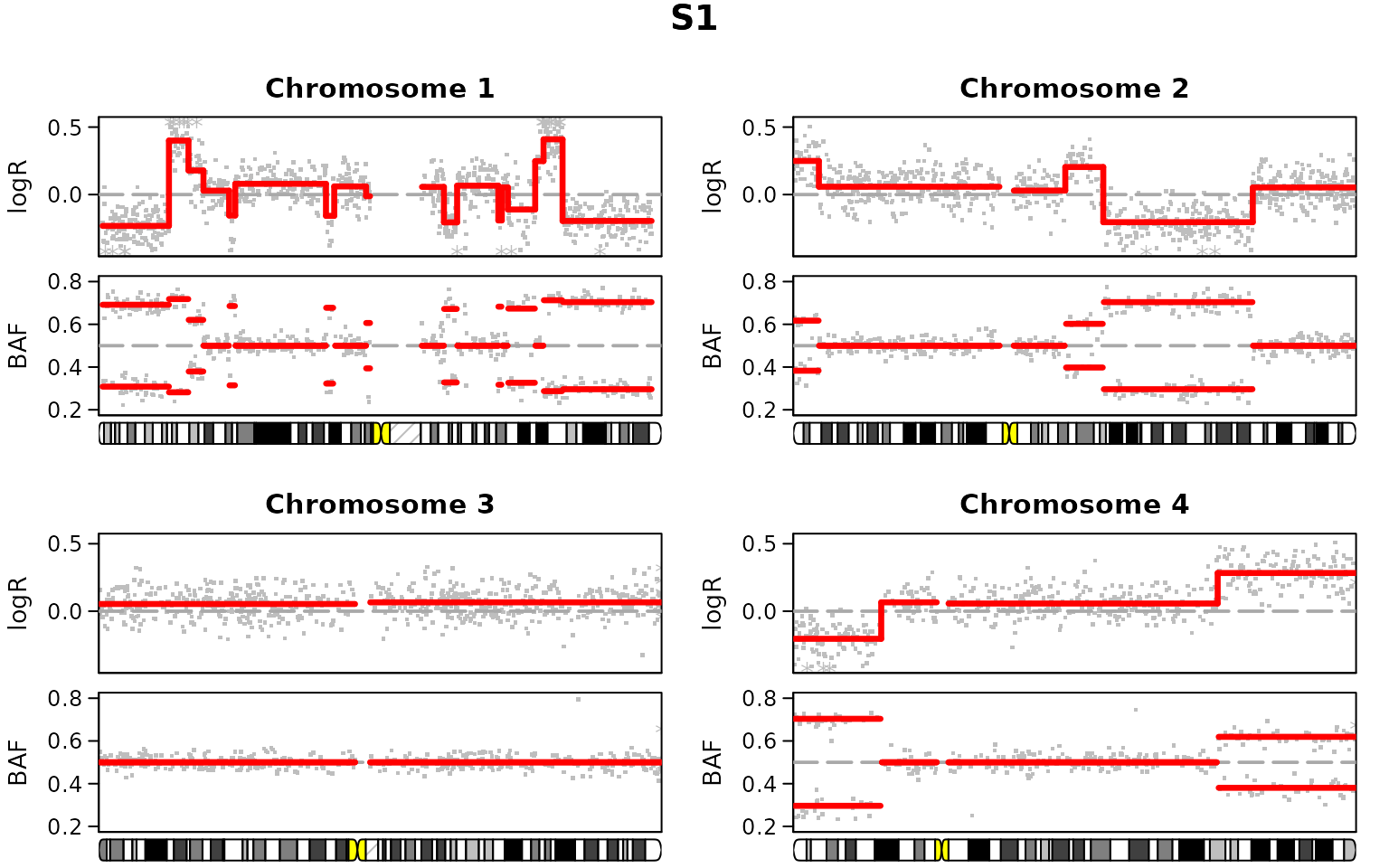

Allele-specific plot for one sample on chromosomes 1-4. Segmentation done by aspcf.

Other graphical tools

Frequency plot

A useful graphical tool is plotFreq, where we plot the frequency of samples in the data set with a gain or a loss at a genomic position. In this example we use pcf to obtain copy number estimates for the entire lymphoma data set:

lymphoma.res <- pcf(data = lymphoma, gamma = 12, verbose = FALSE)

Gains and losses will be regions where the copy number estimate is above or below some defined thresholds specified by the parameters thres.gain and thres.loss, respectively.

plotFreq(segments = lymphoma.res, thres.gain = 0.2, thres.loss = -0.1)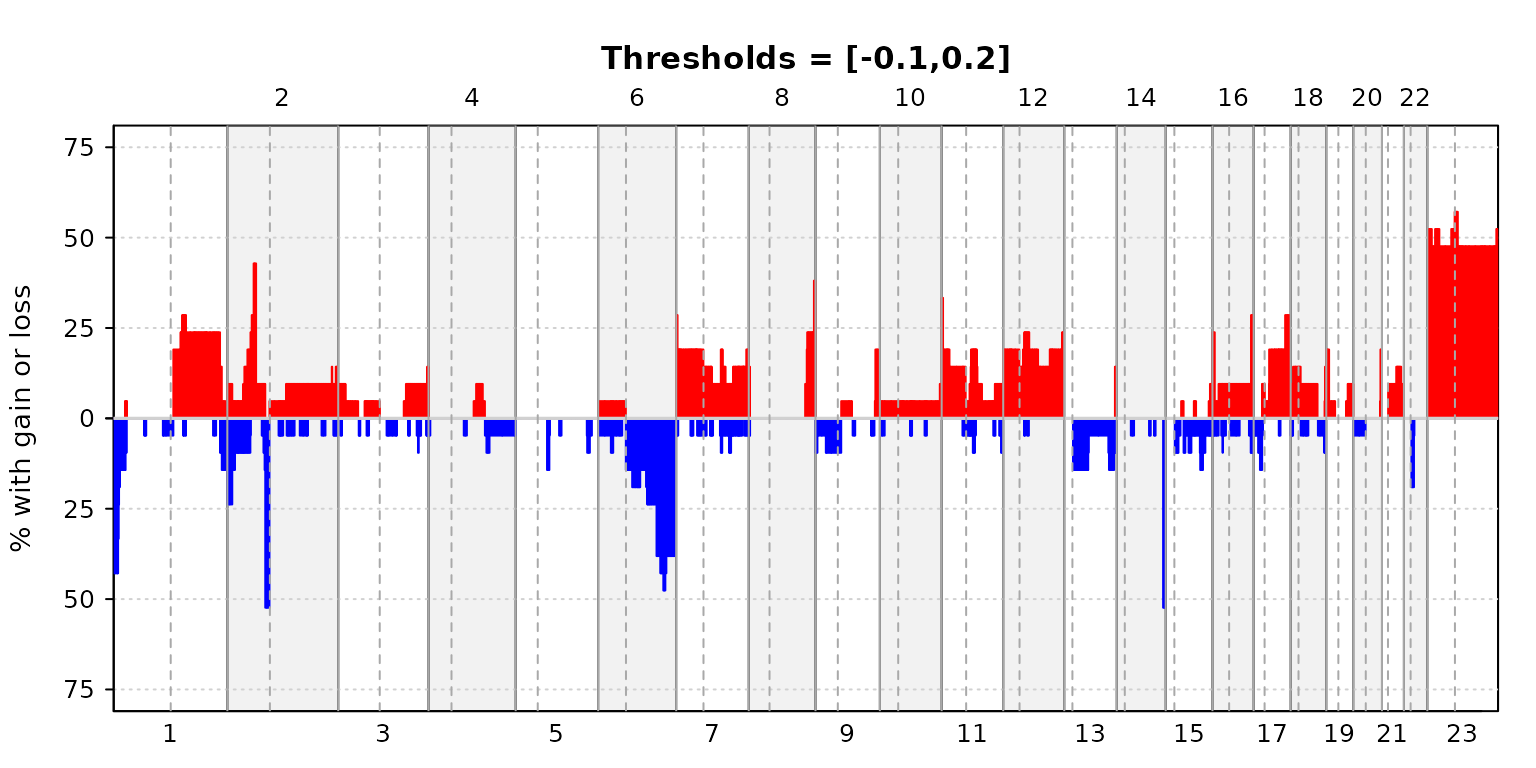

Frequencyplot for lymphoma data

The plot above shows the percentage of samples with estimated $\log_{2}$ copy number ratios above the threshold $0.2$ (gain) in red and below the threshold $-0.1$ (loss) in green. Frequencies may also be plotted per chromosome by specifying chromosomes in the parameter chrom.

Circle plot

A similar plotting routine is plotCircle which also shows the aberration frequencies, but unlike plotFreq the genome is here represented as a circle. The input is again copy number estimates, and aberrations are defined as described above. In addition to plotting aberration frequencies one may show associations between certain genomic regions by specifying the parameter arcs as input. This should be a matrix giving the chromosomes and positions for regions that are connected, as well as a column specifying whether there are different types of associations. One example of use is to plot strong interchromosomal correlations between pairs of segments found by multipcf.

Below, we assume that multipcf has been run on the lymphoma data, and we have calculated the interchromosomal correlations between all segment pairs (see the help file for plotCircle for details). Say strong positive correlations were found between a segment with middle position 168754669 on chromosome 2 and a segment with middle position 61475398 on chromosome 14, as well as between a segment with middle position 847879349 on chromosome 12 and a segment with middle position 30195556 on chromosome 21. In addition, a strong negative correlation was found between a segment with middle position 121809306 on chromosome 4 and a segment with middle position 12364465 on chromosome 17. Having found the location of the associations we want to visualize we can then define the matrix arcs holding the chromosome number and position of a segment in the first two columns, and the chromsome number and position of the associated segment in the next two columns. The fifth column identifies positive correlations and negative correlations as class 1 and 2, respectively:

chr.from <- c(2, 12, 4)
pos.from <- c(168754669, 847879349, 121809306)
chr.to <- c(14, 21, 17)
pos.to <- c(6147539, 301955563, 12364465)
cl <- c(1, 1, 2)
arcs <- cbind(chr.from, pos.from, chr.to, pos.to, cl)

The plot below shows a circle plot. The gain frequencies are shown in red, while loss frequencies are shown in green. In addition, the orange and blue arcs connect the segments which were found to have high positive and negative correlations, respectively.

plotCircle(segments = lymphoma.res, thres.gain = 0.15, arcs = arcs)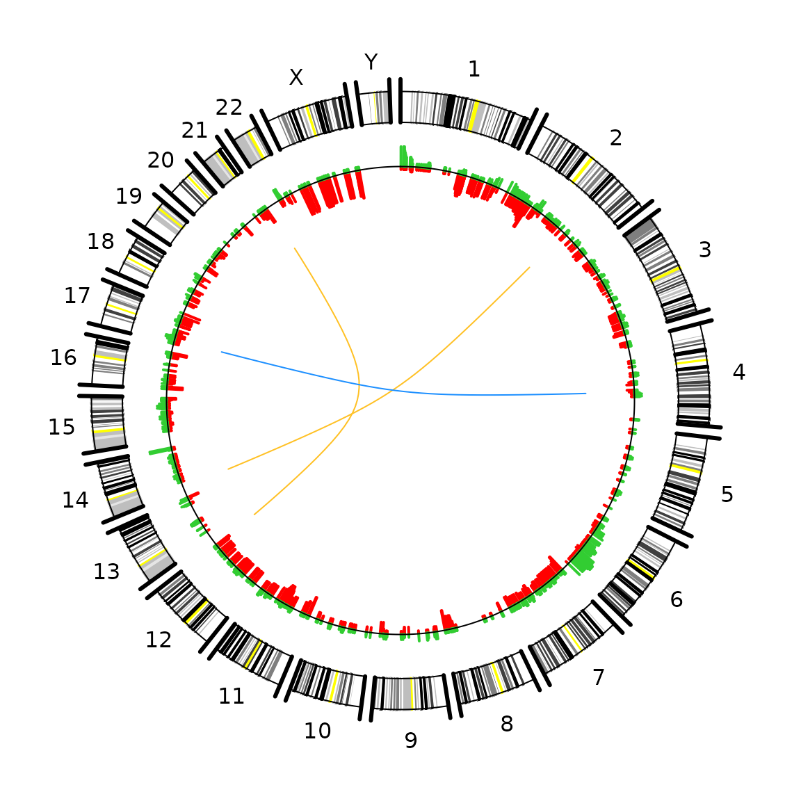

Circle plot for lymphoma data.

Heatmap

Another graphical function is plotHeatmap, which may be used to examine differences between samples. Here a heatmap is plotted for each sample according to the magnitude of the estimated copy number value relative to some pre-defined limits. The plot below shows a heatplot for the lymphoma samples. Each sample is represented by a row. The color red indicates that the estimate is above the upper limit of $0.3$ , while the color blue indicates that it is below the lower limit of $-0.3$ . Darker nuances of red and blue indicate that the value is below and above the upper and lower limit, respectively, and the darker the nuance, the closer the value is to zero.

plotHeatmap(segments = lymphoma.res, upper.lim = 0.3)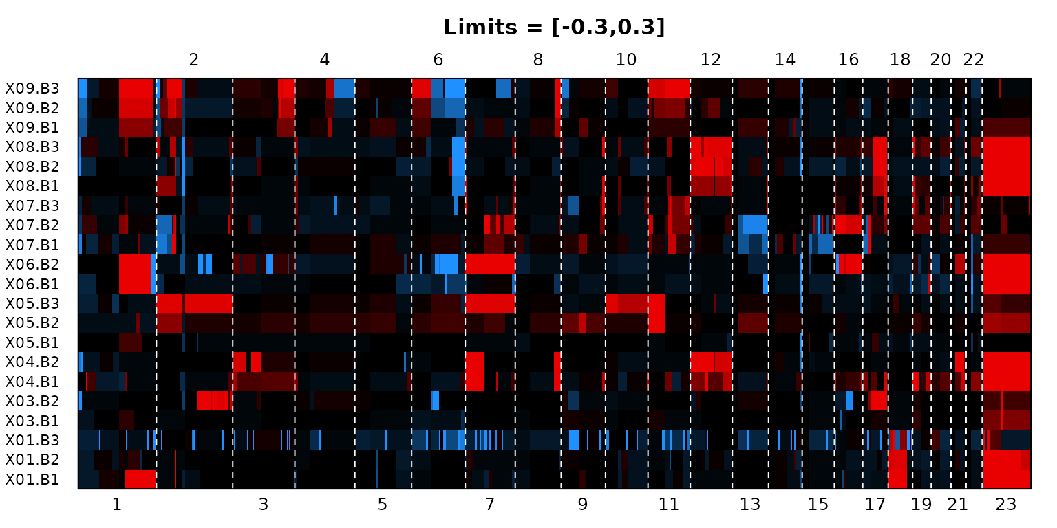

Heatmap for lymphoma data.

Aberration plot

Similarly the function plotAberration is useful for locating recurrent aberrations. An example is given below where each row represents a sample and the colors red and blue indicate gains and losses, respectively.

plotAberration(segments = lymphoma.res, thres.gain = 0.2)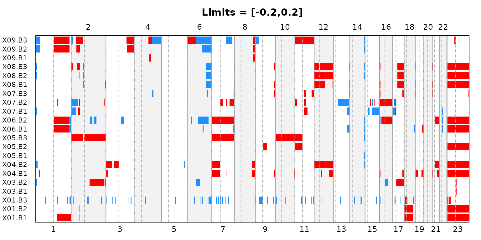

Aberration plot for the lymphoma data.

Diagnostic plot for penalty selection

As mentioned earlier we may apply the function plotGamma to decide on a reasonable choice for the penalty parameter in the segmentation routines. This function will run pcf for a single sample and chromosome using 10 values for gamma in the range indicated by the parameter gammaRange. Each segmentation result is then plotted along with the data in a multigrid plot, and the number of segments found for each value of gamma is shown in the last panel. The plot below gives an example using the first sample in the micma data.

data(micma)
plotGamma(micma, chrom = 17, cex = 3)

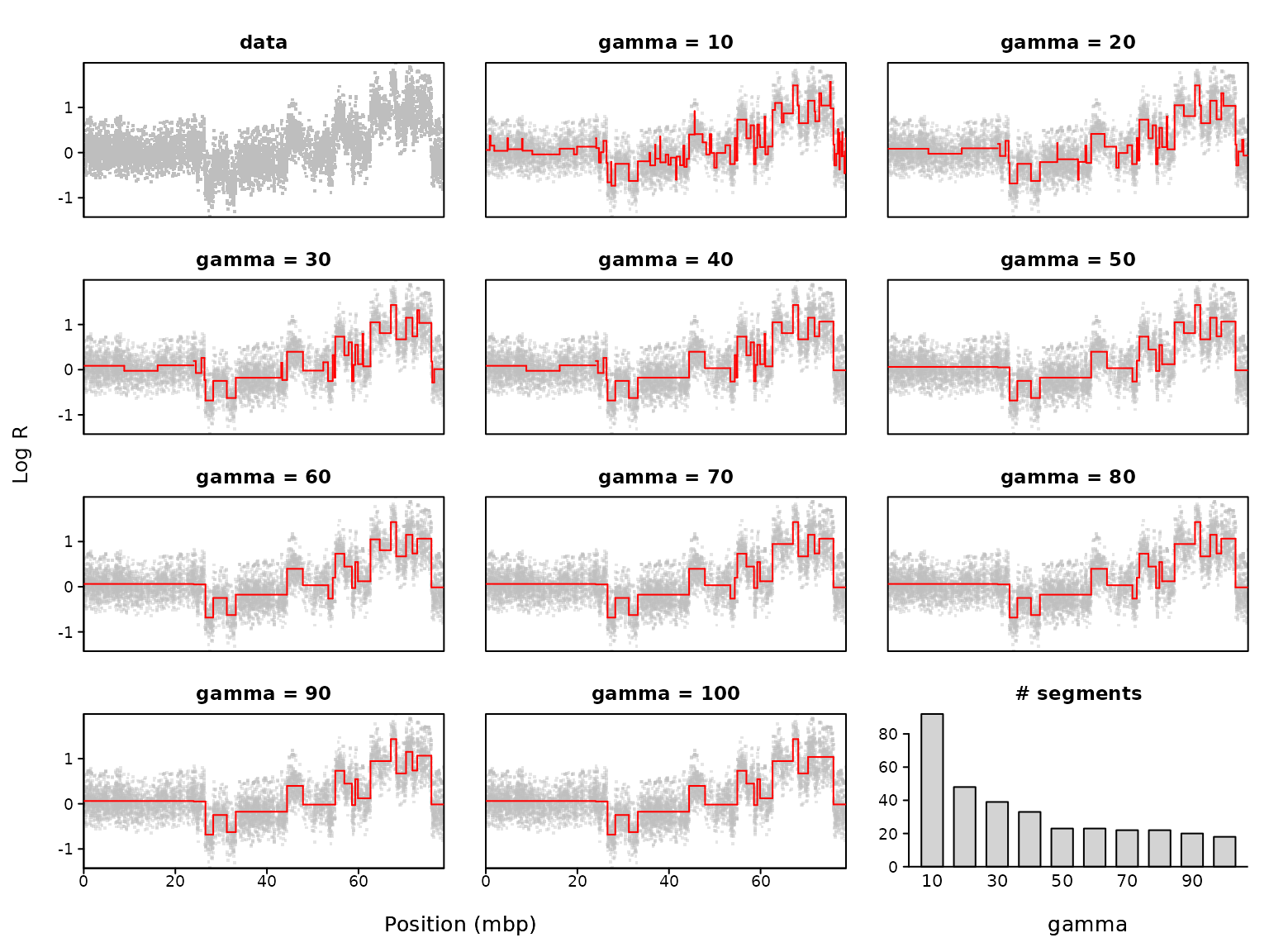
Diagnostic gamma plot for the first sample in the micma data. 10 different gamma-values are evaluated.

An additional option is to specify the parameter cv = TRUE, which means that a 5-fold cross-validation is run for each value of gamma. A graph showing the average residual error from the cross-validation is then added in the last panel of the plot, and the value of gamma which minimizes this error is marked by an asterix. This value may provide a starting point for selecting gamma, but should not be used uncritically because the cross-validation tends to favor too low values and could favor detection of low-amplitude “aberrations” which may be caused by artifacts related to the technology (e.g. due to GC-content).

Tips

When the data set is very large an alternative to specifying the data frame as input in winsorize, pcf, multipcf and aspcf is to supply a txt-file as input in the data parameter. The data txt-file should then be organized in the same way as described for the data earlier, namely with chromosomes and genomic positions in the two first columns, and sample copy number data in all subsequent columns. The data will then be read in and processed chromosome arm by chromosome arm, thus taking up less memory. Similarly, results can be stored in txt-files by setting save.res = TRUE and optionally specifying filenames.

Another way to handle large data sets is by applying the function subsetData to break the data set into a smaller subset only containing certain chromosomes and/or samples. Again, the input may be a data frame or a data txt-file. This function is also useful when plotting the data, and similarly subsetSegments may be used to get a subset of segments for particular chromosomes and/or samples.

If it is not desirable to perform independent segmentations on each chromosome arm, or if the assembly does not match one of hg16-hg19 (e.g. if the data comes from another species), the function pcfPlain can be applied for single-sample segmentation.

In the data/segmentation plots (plotGenome, plotSample, plotChrom, plotAllele) different segmentation results may be visualized together by specifying the input parameter segments as a list. This enables simultaneous examination and comparison of different segmentation results e.g. obtained from pcf and multipcf, or by using different values of gamma. See the help-files for these functions for examples.

Aberration calling for the segments found by pcf or multipcf is done by the function callAberrations. Given user-specified thresholds, this function classifies each segment as normal, gain or loss.

The function selectSegments can be used to retrieve potentially interesting segments found by multipcf. Using this function one may select segments based on a number of characteristics; segments with the largest or smallest variance among the samples, the longest or shortest segments, or the segments that have the largest aberration freqencies.

For the user familiar with the GRanges format from the GenomicRanges package, it is possible to convert the segments data frame via the function getGRangesFormat.

References

Nilsen, G., Liestoel, K., Van Loo, P., Vollan, HKM., Eide, MB., Rueda, OM., Chin, SF., Russel, R., Baumbusch, LO., Caldas, C., Borresen-Dale, AL., Lingjaerde, OC. Copynumber: Efficient algorithms for single- and multi-track copy number segmentation. BMC Genomics 13:591 (2012, doi:10.1186/1471-2164-13-59).

Eide, MB., Liestoel, K., Lingjaerde, OC., Hystad, ME., Kresse, SH., Meza-Zepeda, L., Myklebost O., Troen, G., Aamot, HV., Holte, H., Smeland, EB., Delabie, J. Genomic alterations reveal potential for higher grade transformation in follicular lymphoma and confirm parallell evolution of tumor cell clones. Blood 116 (2010), 1489-1497.

Mathiesen, RR., Fjelldal, R., Liestoel, K., Due, EU., Geigl, JB., Riethdorf, S., Borgen, E., Rye, IH., Schneider, IJ., Obenauf, AC., Mauermann, O., Nilsen, G., Lingjaerde, OC., Borresen-Dale, AL., Pantel, K., Speicher, MR., Naume, B., Baumbusch, LO. High resolution analysis of copy number changes in disseminated tumor cells of patients with breast cancer. Int J Cancer 131(4) (2011), E405-E415.